Section 8: Addressing the limitations of applying Physics in Finance

Log normal Assumption and Market Jumps.

The assumption that asset prices follow a log-normal distribution has been fundamentally challenged by the recurrence of extreme events. As noted, this assumption would not be able to account for the huge crashes in the 2008 recession, the COVID market crash or the 1998 Russian default which proved to be costly for LTCM. Modern finance has attempted to address this issue by integrating jump – diffusion models.

In physics, jump diffusion is used to describe atomic motion in crystalline structures, where atoms move between lattice vacancies in discrete jumps. [1] On longer timescales, this movement averages out to standard diffusion. Techniques such as inelastic neutron scattering and Mössbauer spectroscopy allow scientists to study these microscopic jumps in materials. [2] However, financial jump-diffusion models have no such underlying physical foundation; rather, they are statistical tools constructed to better approximate observed price behaviour.

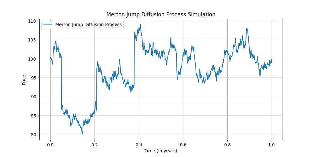
An illustration of this correction is Merton’s jump diffusion model, which he published as an extension to the Black-Scholes model in 1976 [3]. Despite Merton’s contributions to jump-diffusion modelling, there is a distinct irony in the fact that LTCM failed to incorporate the very corrections that could have mitigated its losses. His work extends the Black-Scholes framework by introducing sudden, discrete jumps in asset prices. Mathematically, it is expressed as

$\frac{dS_{t}}{S_{t}} = ( \mu - \lambda k)dt + \sigma dW_{t}+dQ_{t}$ ,

where:

$\lambda$ : The jump intensity – representing the average jumps per time following a poison distribution.

$k$ : The expected relative jump size, given by: $k=E(Y_{i} - 1)$ where $Y_{i}$ follows a log-normal distribution.

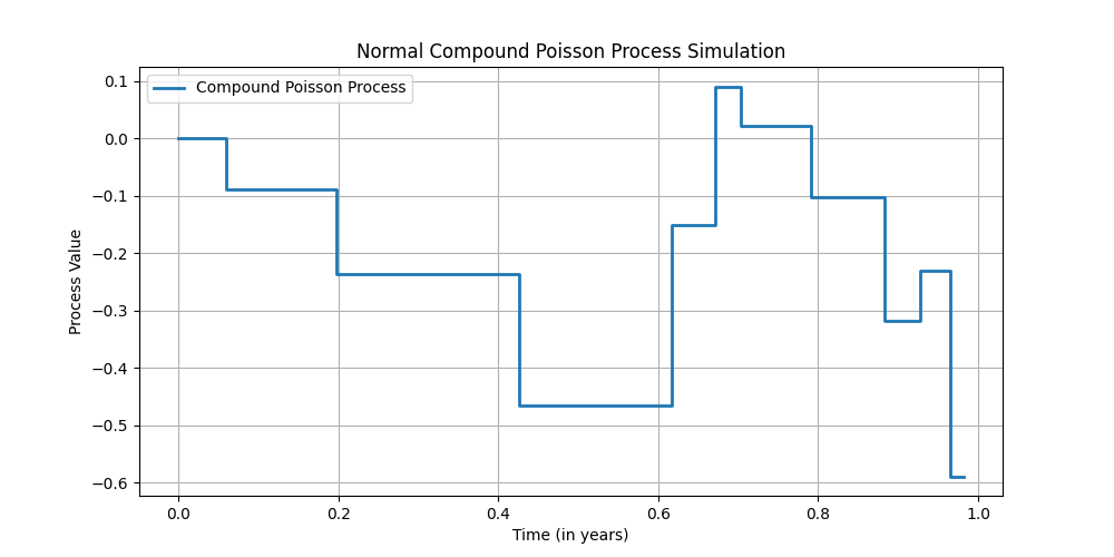
$Q_{t}$ : A compound Poisson process, summing all price jumps over time:

$Q_{t} = \sum_{i=1}^{N_{i}} {Y_{i}-1$

where represents the number of jumps up to time $t$ .

The key distinction from the Black-Scholes model is that this formulation allows for sudden, large changes in asset prices, rather than assuming smooth, continuous changes driven only by Brownian motion. This additional term introduces fat-tailed behaviour in asset returns, helping to better approximate real-world financial data.

Figure 1: Comparison of a Normal Compound Poisson Process (stepwise jumps) and a Merton Jump Diffusion Process (continuous evolution with occasional jumps) in financial modelling.

Moving Beyond Constant Volatility: Stochastic Volatility Models

One clear flaw in the Black – Scholes model is the assumption of a constant volatility parameter. To correct this, stochastic volatility models such as Heston Model introduces a second stochastic process governing volatility itself. It can be derived using the following steps:

1) The Heston model assumes that the asset price $S_{t}$ follows the following stochastic differential equation (SDE):

$dS_{t} = \mu S_{t} + \sqrt{v_{t}} S_{t} d W^{S}_{t}$

Where:

$\mu$ is the drift rate of the asset price,
$v_{t}$ is the variance or volatility squared
$W^{S}_{t}$ is a Wiener process driving the asset price.

The variance $v_{t}$ evolves according to another SDE:

$dv_{t} = \kappa (\theta - v_{t}) dt + \sigma_{v} \sqrt{v_{t}} d W^{v}_{t}$

Where:

$\kappa$ is the rate of mean reversion of the volatility to the long-term mean $\theta$
$\sigma_{v}$ is the volatility of the volatility
$W^{v}_{t}$ is the Wiener process driving the volatility process.

2) Correlation between Asset Price and Volatility

In the Heston Model, the Brownian motions driving $S_{t}$ and $v_{t}$ are assumed to be correlated. The correlation between $d W^{S}_{t}$ and $d W^{v}_{t}$ is denoted as $\rho$ and it is assumed that:

$\mathbb{E} [d W^{S}_{t} d W^{v}_{t}] = \rho dt$

This follows the same Ito’s Calculus used in the derivation of the BS model. This correlation is important because it allows for volatility to rise when the asset price drops, which reflects the “leverage effect” observed in financial markets.

3) Deriving the Characteristic Function (the expectation of the complex exponential of $S_t$ )

The Heston model does not have a closed-form solution for option pricing, but it provides an analytical solution [4] for the characteristic function of the asset price. The characteristic function $\phi (u,t)$ is useful for obtaining option prices through Fourier inversion methods. The characteristic function for the Heston model is derived using the fact that the solution to the SDE for $S_{t}$ can be written in terms of a Fourier transform.

The characteristic function of the asset price under the Heston model is:

$\phi (u,t) = exp([iulog S_{0} + (iu \mu - \frac{1}{2} u^{2}) v_{0} ] t +$ terms involving $\kappa$ , $\sigma_{v}$ , $\theta$ , $\rho$ $)$

Where this expression accounts for the volatility process and the correlation between the asset price and volatility.

4) Option Pricing via Fourier Transform

To calculate the option price, we use the Fourier transform method. The price of a European call option $C(S_{0}, T)$ at time $T$ is given by:

$C(S_{0}, T) = \frac{1}{2 \pi} \int_{-\infty}^{+\infty}exp(iu log S_{0}) \hat{C} (u,T)\,du$

Where $\hat{C} (u,T)$ is the Fourier Transform of the payoff function. For a European call option, the payoff function is $max(S_{T} - K, 0)$ where $K$ is the strike price of the option.

Dynamic Interest Rate Models: Fixing the Constant Rate Assumption

The Black-Scholes framework also assumes a fixed risk-free interest rate, an oversimplification that ignores the impact of monetary policy, inflation, and economic shifts. In reality, these interest rates fluctuate greatly. To address this, stochastic interest rate models such as Vasicek and Cox-Ingersoll-Ross (CIR) introduce:

Random fluctuations: Instead of a constant rate, these models include a stochastic term (a Wiener process) that captures uncertainty in rate movements, allowing rates to evolve dynamically. [5]
Volatility-dependent behaviour: The CIR model prevents negative interest rates by making volatility proportional to the square root of the rate, a mathematical fix that reflects how real-world rates behave under economic constraints. [6]

These stochastic models replace the incorrect assumption of constant parameters with formulations that align with observed market behaviour, ensuring more accurate pricing and risk assessment. Again, their existence shows that implementing physical equations often need significant fine tuning to be applicable.

References :

[1] Chudley, C.T. and Elliott, R.J., 1961. Neutron scattering from a liquid on a jump diffusion model. Proceedings of the Physical Society, 77(2), p.353. https://doi.org/10.1088/0370-1328/77/2/319

[2] Vogel, G., 1999. Recent studies on diffusion in intermetallics by mossbauer spectroscopy and nuclear resonant scattering of synchrotron radiation. High Temperature Materials and Processes, 18(5-6), pp.293-304. https://doi.org/10.1515/htmp.1999.18.5-6.293

[3] Merton, R.C., 1976. Option pricing when underlying stock returns are discontinuous. Journal of financial economics, 3(1-2), pp.125-144. https://doi.org/10.1016/0304-405x(76)90022-2

[4] Hull, J.C. and Basu, S., 2016. Options, futures, and other derivatives. Pearson Education India. pp.625 https://doi.org/10.23874/amber/2016/v7/i1/121351

[5] Lin, J., Liao, G., Chen, M. and Yin, H., 2021. Two-phase degradation modeling and remaining useful life prediction using nonlinear wiener process. Computers & Industrial Engineering, 160, p.107533. https://doi.org/10.1016/j.cie.2021.107533

[6] Orlando, G., Mininni, R.M. and Bufalo, M., 2018. On The Calibration of Short-Term Interest Rates Through a CIR Model. arXiv preprint https://arxiv.org/pdf/1806.03683 [accessed 21/02/2025]