
Brownian Motion
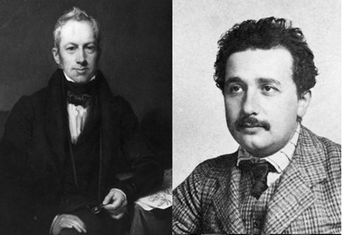
Brownian motion was discovered by 19th century botanist Robert Brown. Whilst examining pollen grains suspended in water under a microscope, Brown observed tiny particles that had been ejected by the pollen grains exhibiting continuous, jittery motion [1]. Though Brown ascertained that this motion was not biological in origin, it took until 1905 for Albert Einstein to apply molecular theory and explain Brownian motion as a stochastic Wiener process [2].

The motion Brown observed was a three-dimensional random walk. Einstein theorised that the ejected particles were surrounded by millions of minuscule invisible atoms [3]. At the turn of the 20th century, atoms were considered to be more a useful mathematical trick than a physical reality by most of the scientific community, despite notable proponents including Ludwig Boltzmann, who himself made major contributions to statistical thermodynamics and the understanding of thermodynamical systems as stochastic processes. Einstein, however, believed atoms to be a physical reality, and that Brownian motion was caused by the collision between the ejected particles and millions of atoms at any given time. To describe this motion mathematically, Einstein assumed that due to the complexity of the collisions, at any given time a particle had an equal probability to move in any direction in 3-dimensional space, regardless of its previous motion. Brownian motion is therefore described as a 3-dimensional Wiener process, and experimental evidence had been provided to prove that atoms were indeed a physical reality.
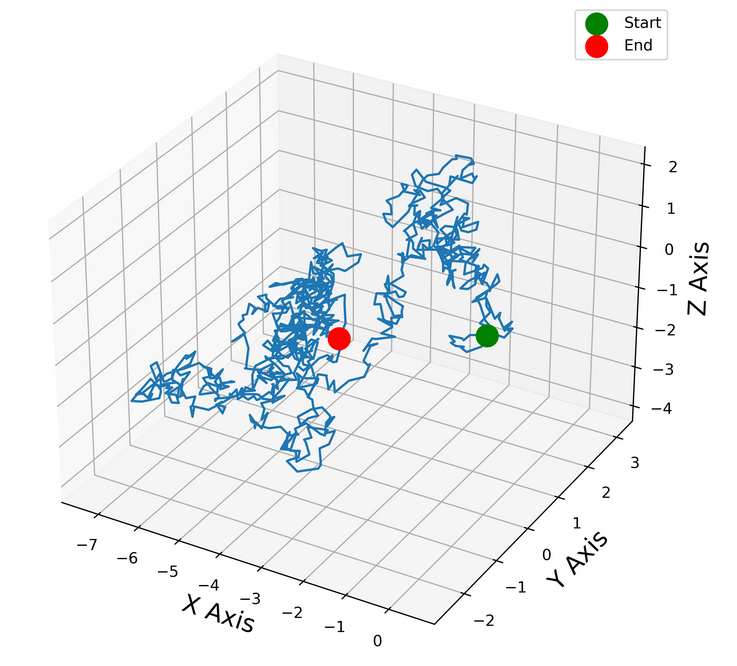
Simulation of a particle undergoing 3-D Brownian motion.
When modelling the fluctuation in an assets value as Brownian motion, we make a similar assumption to that made by Einstein: at any time, a stock has a 50/50 change to increase or decrease in value. There are key differences between a simple random walk and Brownian motion. In the section Stochastic Processes, the random walks implemented were Gaussian; we measured the motion of the walkers’ discrete time intervals, each step, and in discrete space, with each step moving a walker exactly plus or minus one unit. Brownian motion on the other hand is a Wiener process measured in continuous space and time. In the context of finance this may seem counter-intuitive: we cannot sell as stock for £𝜋, and the price of a stock cannot be updated at infinitesimal time increments. However, the benefits of modelling the fluctuation in asset price as Brownian motion, introducing randomness into financial models, outweighs the unrealistic assumptions of the model.
Geometric Brownian Motion
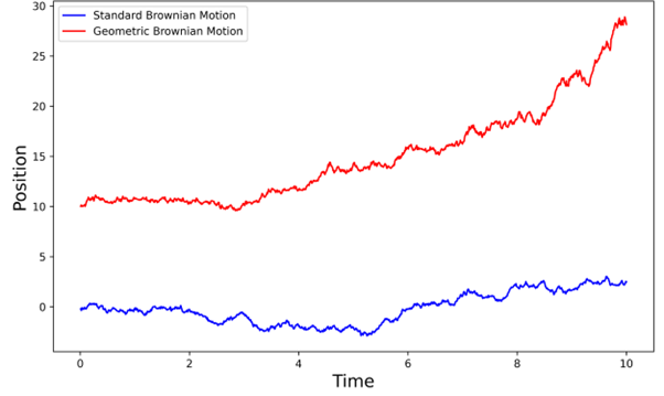
Standard models of Brownian motion bear strong similarities to the random fluctuations of an assets’ value but there are key differences in the behaviour of stock prices and standard simple Brownian motion. In simple Brownian motion, the position a particle takes can be negative, but the price of an asset cannot take a negative value. Moreover, whereas the mean position of a large group of particles undergoing Brownian motion will be zero, the value of assets globally exhibit an overall exponential growth over time, that has been empirically measured for centuries. To resolve these issues, the standard Brownian motion model must be revised and into a model called geometric Brownian motion [4].
Geometrical Brownian motion is a stochastic process modelled by the following differential equation:

In the context of finance, S is the price of an asset, μ the expected growth rate of the asset and introduces exponential growth over long timescales, σ the volatility of value of the asset and W is the simple model of Brownian motion, called a Wiener process, encoding the randomness of the system. This model better simulates the long-term growth of asset values whilst still maintaining the intrinsic small-scale randomness in the value of an asset.
Mu Slider
Sigma Slider
Modelling the price of an asset using geometrical Brownian motion has numerous advantages. The model maintains that the expected returns on an asset are independent of its’ initial price, the key motivation of modelling markets as stochastic processes. It is also relatively simple to solve the equation for geometric Brownian motion, which is useful when applying them in financial models. However, geometric Brownian motion relies on there being a constant volatility in the value of the asset σ, whereas in the real world the volatility of assets is dependent on current market conditions and therefore variable. The growth rate μ is also assumed to be constant, meaning the model cannot account for extended periods of accelerated or slow growth in the value of an asset. Importantly, these two assumptions mean that models built around geometric Brownian motion cannot adequately model shocks in the stock market which cause the value of assets to jump dramatically, such as the 2008 global financial crisis that dramatically altered global values almost instantaneously.
Geometric Brownian incorporates the standard model of Brownian motion to model a stochastic process that on small timescales behaves randomly with a constant volatility σ but exhibits long term exponential growth with a constant growth rate μ. Financial models built upon geometric Brownian motion can model the normal activity of markets with accuracy but are limited by being unable to model the impacts of shocks to the market. The most significant application of geometrical Brownian motion in finance is the Black-Scholes model, developed by Fischer Black and Myron Scholes and extended by Robert C. Merton and used to value the price of an option.