What is a Stochastic Process?
A stochastic process, put simply, is a random process. Stochastic processes are ubiquitous in nature; the spontaneous decay of radioactive particles, the diffusion of gas particles and the growth of a bacteria culture are all examples of stochastic processes in science. In recent years stochastic processes have been discovered in the movements of animals through an ecosystem and in the neural pathways of the brain, highlighting the pervasiveness of stochastic processes in countless fields of research.
The fundamental characteristic of all stochastic processes is that the past behaviour of the system cannot be used to predict the future behaviour of the system. For example, if we were to play heads or tails and flip heads four times in a row, we still would have an exactly 50/50 chance of flipping tails on the fifth go. The previous behaviour of the coin has no influence on subsequent outcomes.
Mathematically, a stochastic process is defined as a collection of random variables indexed by a mathematical set, with each variable being uniquely associated with an element of that set [1]. In most real-world applications of stochastic processes, the set is a series of points in time, with each random variable being indexed as the state of the system at that time. A stochastic process can be measured at discrete time intervals, called a Gaussian process, or continuously, called a Wiener process, and can be measured in numerous spatial dimensions. Geometric Brownian motion, the type of stochastic motion modelled in the Black-Scholes equation, is a 1-dimensional Wiener process, also called a random walk.
Random Walks
One of the simplest examples of a stochastic process is a 1-dimensional random walk. A random walk is the path taken due to a sequence of random steps in space.
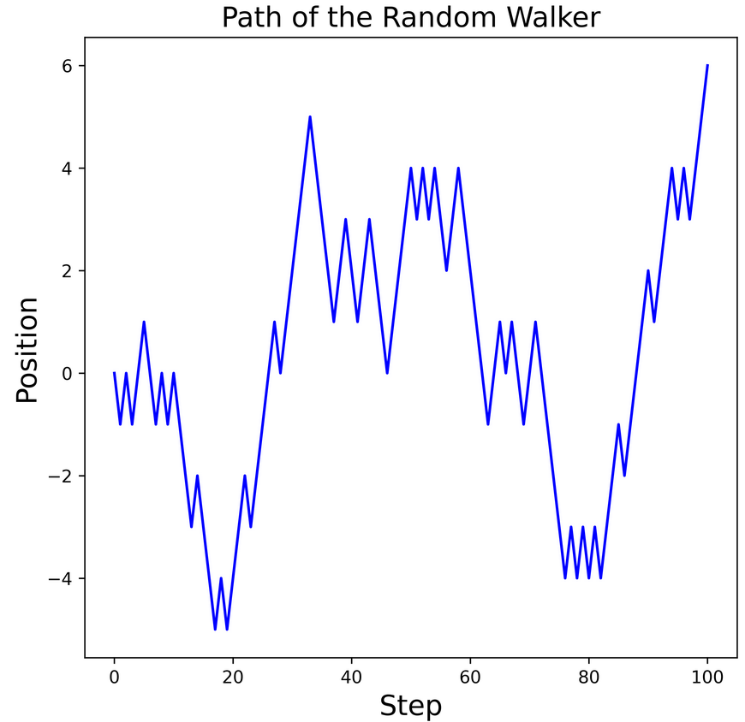
Consider a random walker who at each step has two options: to move forwards (in the positive direction) by one unit, or to move backwards (in the negative direction) by one unit. The walker has an equal probability to move forwards or backwards at each step.
If the path of the random walker over is simulated over 100 steps, we observe random motion: there is no overall pattern to the walkers’ movements. If a further 100 steps were simulated and the axes were removed, it would be impossible to tell which steps came first, as the previous behaviour of the walker does not influence their subsequent path. If the random walker was simulated over an infinite number of steps, the walker would visit every point in 1-d space and would take every possible path over a finite number of steps.
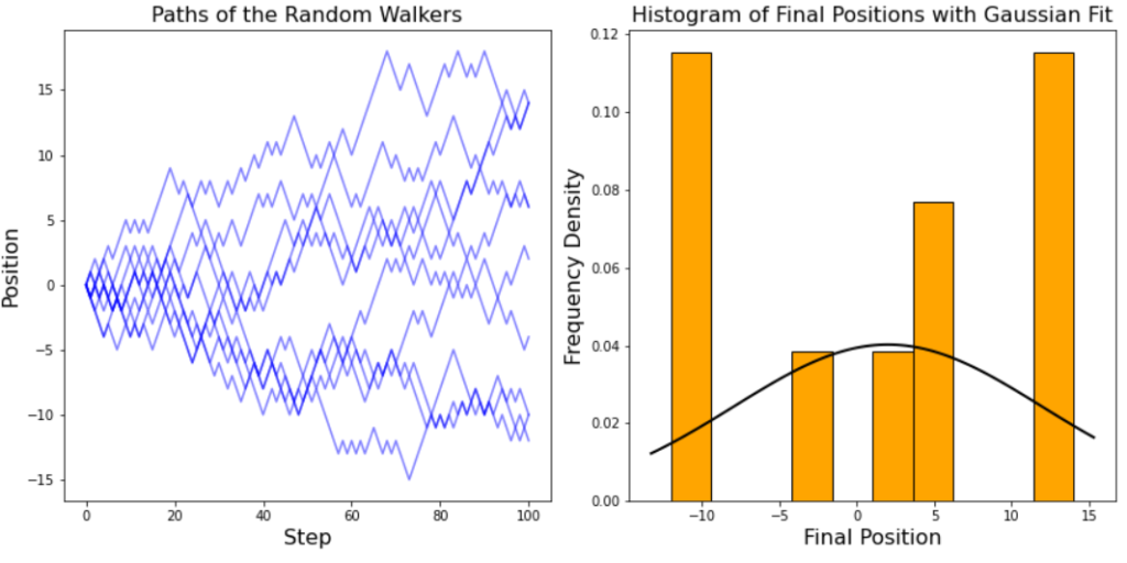
If we simulate the paths of 10 random walkers, we see that there is no pattern to their final positions. However, if the number of walkers increases to 100, the final positions of the walkers begin to take the shape of a normal distribution.
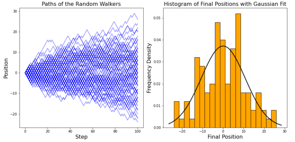
If the number of walkers increases to 1000, the normal distribution of the final positions of the walkers is clear to see.
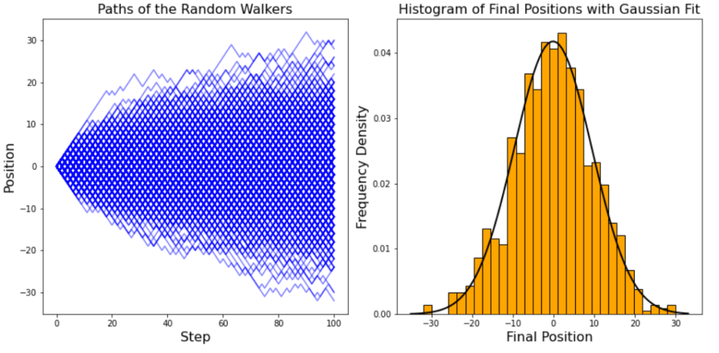
The final positions of the walkers obey a normal distribution, which has several important properties. The distribution of final positions is symmetrical about a mean value of zero, each walkers starting position. Intuitively this makes sense: there is an equal chance of the walkers moving in the positive and negative directions, so there is no overall preference towards a positive or negative final position. The densest region of the distribution are the positions close to zero. This is because there are many possible paths a walker can take to reach a final position of around zero, whereas positions at the extremities of the distribution have relatively few paths a particle can take to reach them. For a particle to reach a final position of 100, they must move forward at each of their 100 steps, with a probability of under 1 in 1030. As the number of walkers increases, the range of the final positions increases due to more opportunities for the walkers to take unlikely paths towards the extremities of the distribution. We can also measure the spread in the data, the standard deviation, which describes the range enclosing the middle 67% of the data.
This simple example of stochastic motion shows that despite each random walk being intrinsically random, simulating many random walks allows properties of the system to be measured. Not all stochastic processes obey the normal distribution as shown above; the number of radioactive particles that decay in a time interval is modelled by an alternative distribution, the Poisson distribution. All stochastic processes are described by some probabilistic distribution, from which properties of the system can be discerned.
Random Walk Simulation
Progress: 0 / 500